Advanced

The basic interface explained in the Introduction should provide you enough to start detecting communities. However, perhaps you want to improve the partitions further or want to do some more advanced analysis. In this section, we will explain this in more detail.

Optimiser

Although the package provides simple access to the function find_partition(), there is actually an underlying Optimiser class that is doing the actual work. We can also explicitly construct an Optimiser object:

>>> optimiser = la.Optimiser()

The function find_partition() then does nothing else then calling optimise_partition() on the provided partition.

>>> diff = optimiser.optimise_partition(partition)

optimise_partition() simply tries to improve any provided partition. We can thus try to repeatedly call optimise_partition() to keep on improving the current partition:

>>> G = ig.Graph.Erdos_Renyi(100, p=5./100)
>>> partition = la.ModularityVertexPartition(G)
>>> diff = 1
>>> while diff > 0:
...   diff = optimiser.optimise_partition(partition)

Even if a call to optimise_partition() did not improve the current partition, it is still possible that a next call will improve the partition. Of course, if the current partition is already optimal, this will never happen, but it is not possible to decide whether a partition is optimal.

This functionality of repeating multiple iterations is actually already built-in. You can simply call

>>> diff = optimiser.optimise_partition(partition, n_iterations=10)

If n_iterations < 0 the optimiser continues iterating until it encounters an iterations that did not improve the partition.

The optimise_partition() itself is built on two other basic algorithms: move_nodes() and merge_nodes(). You can also call these functions yourself. For example:

>>> diff = optimiser.move_nodes(partition)

or

>>> diff = optimiser.merge_nodes(partition)

The simpler Louvain algorithm aggregates the partition and repeats the move_nodes() on the aggregated partition. We can easily emulate that:

>>> partition = la.ModularityVertexPartition(G)
>>> while optimiser.move_nodes(partition) > 0:
...   partition = partition.aggregate_partition()

This summarises the whole Louvain algorithm in just three lines of code. Although this finds the final aggregate partition, it leaves unclear the actual partition on the level of the individual nodes. In order to do that, we need to update the membership based on the aggregate partition, for which we use the function from_coarse_partition().

>>> partition = la.ModularityVertexPartition(G)
>>> partition_agg = partition.aggregate_partition()
>>> while optimiser.move_nodes(partition_agg) > 0:
...   partition.from_coarse_partition(partition_agg)
...   partition_agg = partition_agg.aggregate_partition()

Now partition_agg contains the aggregate partition and partition contains the actual partition of the original graph G. Of course, partition_agg.quality() == partition.quality() (save some rounding).

Instead of move_nodes(), you could also use merge_nodes(). These functions depend on choosing particular alternative communities: the documentation of the functions provides more detail.

One possibility is that rather than aggregating the partition based on the current partition, you can first refine the partition and then aggregate it. This is what is done in the Leiden algorithm, and can be done using the functions move_nodes_constrained() and merge_nodes_constrained(). Implementing this, you end up with the following high-level implementation of the Leiden algorithm:

>>> # Set initial partition
>>> partition = la.ModularityVertexPartition(G)
>>> refined_partition = la.ModularityVertexPartition(G)
>>> partition_agg = refined_partition.aggregate_partition()
>>>
>>> while optimiser.move_nodes(partition_agg):
...
...   # Get individual membership for partition
...   partition.from_coarse_partition(partition_agg, refined_partition.membership)
...
...   # Refine partition
...   refined_partition = la.ModularityVertexPartition(G)
...   optimiser.merge_nodes_constrained(refined_partition, partition)
...
...   # Define aggregate partition on refined partition
...   partition_agg = refined_partition.aggregate_partition()
...
...   # But use membership of actual partition
...   aggregate_membership = [None] * len(refined_partition)
...   for i in range(G.vcount()):
...     aggregate_membership[refined_partition.membership[i]] = partition.membership[i]
...   partition_agg.set_membership(aggregate_membership)

These functions in turn rely on two key functions of the partition: diff_move() and move_node(). The first calculates the difference when moving a node, and the latter actually moves the node, and updates all necessary internal administration. The move_nodes() then does something as follows

>>> for v in G.vs:
...   best_comm = max(range(len(partition)),
...                   key=lambda c: partition.diff_move(v.index, c))
...   partition.move_node(v.index, best_comm)

The actual implementation is more complicated, but this gives the general idea.

This package builds on a previous implementation of the Louvain algorithm in louvain-igraph. To illustrate the difference between louvain-igraph and leidenalg, we ran both algorithms for 10 iterations on a Youtube network of more than 1 million nodes and almost 3 million edges.

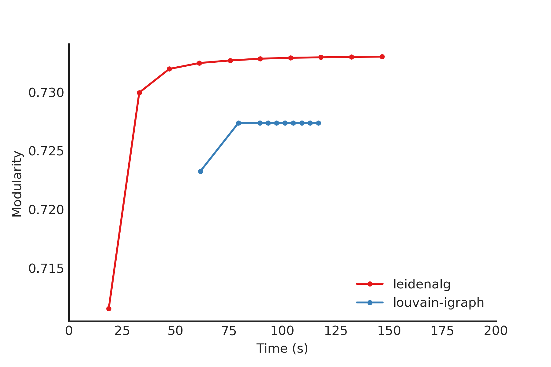
The results are quite clear: Leiden is able to achieve a higher modularity in less time. It also points out that it is usually a good idea to run Leiden for at least two iterations; this is also the default setting.

Note that even if the Leiden algorithm did not find any improvement in this iteration, it is always possible that it will find some improvement in the next iteration.

Resolution profile

Some methods accept so-called resolution parameters, such as CPMVertexPartition or RBConfigurationVertexPartition. Although some methods may seem to have some ‘natural’ resolution, in reality this is often quite arbitrary. However, the methods implemented here (which depend in a linear way on resolution parameters) allow for an effective scanning of a full range for the resolution parameter. In particular, these methods somehow can be formulated as \(Q = E - \gamma N\) where \(E\) and \(N\) are some other quantities. In the case for CPMVertexPartition for example, \(E = \sum_c m_c\) is the number of internal edges and \(N = \sum_c \binom{n_c}{2}\) is the sum of the internal possible edges. The essential insight for these formulations [1] is that if there is an optimal partition for both \(\gamma_1\) and \(\gamma_2\) then the partition is also optimal for all \(\gamma_1 \leq \gamma \leq \gamma_2\).

Such a resolution profile can be constructed using the Optimiser object.

>>> G = ig.Graph.Famous('Zachary')
>>> optimiser = la.Optimiser()
>>> profile = optimiser.resolution_profile(G, la.CPMVertexPartition,
...                                        resolution_range=(0,1))

Plotting the resolution parameter versus the total number of internal edges we thus obtain something as follows:

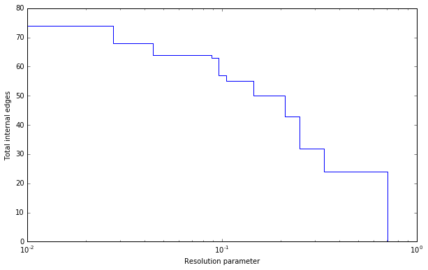
Now profile contains a list of partitions of the specified type (CPMVertexPartition in this case) for resolution parameters at which there was a change. In particular, profile[i] should be better until profile[i+1], or stated otherwise for any resolution parameter between profile[i].resolution_parameter and profile[i+1].resolution_parameter the partition at position i should be better. Of course, there will be some variations because optimise_partition() will find partitions of varying quality. The change points can then also vary for different runs.

This function repeatedly calls optimise_partition() and can therefore require a lot of time. Especially for resolution parameters right around a change point there may be many possible partitions, thus requiring a lot of runs.

Fixed nodes

For some purposes, it might be beneficial to only update part of a partition. For example, perhaps we previously already ran the Leiden algorithm on some dataset, and did some analysis on the resulting partition. If we then gather new data, and in particular new nodes, it might be useful to keep the previous community assignments fixed, while only updating the community assignments for the new nodes. This can be done using the is_membership_fixed argument of find_partition(), see [2] for some details.

For example, suppose we previously detected partition for graph G, which was extended to graph G2. Assuming that the previously exiting nodes are identical, we could create a new partition by doing

>>> new_membership = list(range(G2.vcount()))
... new_membership[:G.vcount()] = partition.membership

We can then only update the community assignments for the new nodes as follows

>>> new_partition = la.CPMVertexPartition(G2, new_membership,
...                                       resolution_parameter=partition.resolution_parameter)
... is_membership_fixed = [i < G.vcount() for i in range(G2.vcount())]
>>> diff = optimiser.optimise_partition(new_partition, is_membership_fixed=is_membership_fixed)

In this example we used CPMVertexPartition. but any other VertexPartition would work as well.

Maximum community size

In some cases, you may want to restrict the community sizes. It is possible to indicate this by setting the max_comm_size parameter so that this constraint is taken into account during optimisation. In addition, it is possible to pass this parameter directly when using find_partition(). For example

>>> partition = la.find_partition(G, la.ModularityVertexPartition, max_comm_size=10)

References

[1]

Traag, V. A., Krings, G., & Van Dooren, P. (2013). Significant scales in community structure. Scientific Reports, 3, 2930. 10.1038/srep02930

[2]

Zanini, F., Berghuis, B. A., Jones, R. C., Robilant, B. N. di, Nong, R. Y., Norton, J., Clarke, Michael F., Quake, S. R. (2019). northstar: leveraging cell atlases to identify healthy and neoplastic cells in transcriptomes from human tumors. BioRxiv, 820928. 10.1101/820928