Multiplex
The implementation of multiplex community detection builds on ideas in [1]. The most basic form simply considers two or more graphs which are defined on the same vertex set, but which have differing edge sets. In this context, each node is identified with a single community, and cannot have different communities for different graphs. We call this layers of graphs in this context. This format is actually more flexible than it looks, but you have to construct the layer graphs in a smart way. Instead of having layers of graphs which are always identified on the same vertex set, you could define slices of graphs which do not necessarily have the same vertex set. Using slices we would like to assign a node to a community for each slice, so that the community for a node can be different for different slices, rather than always being the same for all layers. We can translate slices into layers but it is not an easy transformation to grasp fully. But by doing so, we can again rely on the same machinery we developed for dealing with layers.
Throughout the remained of this section, we assume an optimiser has been created:
>>> optimiser = la.Optimiser()
Layer multiplex
If we have two graphs which are identified on exactly the same vertex set, we
say we have two layers. For example, suppose graph G_telephone contains
the communication between friends over the telephone and that the graph
G_email contains the communication between friends via mail. The exact same
vertex set then means that G_telephone.vs[i] is identical to the node
G_email.vs[i]. For each layer we can separately specify the type of
partition that we look for. In principle they could be different for each
layer, but for now we will assume the type of partition is the same for all
layers. The quality of all partitions combined is simply the sum of the
individual qualities for the various partitions, weighted by the
layer_weight. If we denote by \(q_k\) the quality of layer \(k\)
and the weight by \(w_k\), the overall quality is then
The optimisation algorithm is no different from the standard algorithm. We simply calculate the overall difference of moving a node to another community as the sum of the individual differences in all partitions. The rest (aggregating and repeating on the aggregate partition) simple proceeds as usual.
The most straightforward way to use this is then to use
find_partition_multiplex():
>>> membership, improv = la.find_partition_multiplex(
...                        [G_telephone, G_email],
...                        la.ModularityVertexPartition);
Note
You may need to carefully reflect how you want to weigh the importance
of an individual layer. Since the ModularityVertexPartition
is normalised by the number of links, you essentially weigh layers the same,
independent of the number of links. This may be undesirable, in which case it
may be better to use RBConfigurationVertexPartition, which is
unnormalised. Alternatively, you may specify different layer_weights.
Similar to the simpler function find_partition(), it is a simple
helper function. The function returns a membership vector, because the
membership for all layers is identical. You can also control the partitions and
optimisation in more detail. Perhaps it is better to use
CPMVertexPartition with different resolution parameter for
example for different layers of the graph. For example, using email creates a
more connected structure because multiple people can be involved in a single
mail, which may require a higher resolution parameter for the email graph.
>>> part_telephone = la.CPMVertexPartition(
...                    G_telephone, resolution_parameter=0.01);
>>> part_email = la.CPMVertexPartition(
...                    G_email, resolution_parameter=0.3);
>>> diff = optimiser.optimise_partition_multiplex(
...                    [part_telephone, part_email]);
Note that part_telephone and part_email contain exactly the same
partition, in the sense that part_telephone.membership ==
part_email.membership. The underlying graph is of course different, and hence
the individual quality will also be different.
Some layers may have a more important role in the partition and this can be
indicated by the layer_weight. Using half the weight for the email layer for
example would be possible as follows:
>>> diff = optimiser.optimise_partition_multiplex(
...   [part_telephone, part_email],
...   layer_weights=[1,0.5]);
Negative links
The layer weights are especially useful when negative links are present,
representing for example conflict or animosity. Most methods (except CPM) only
accept positive weights. In order to deal with graphs that do have negative
links, a solution is to separate the graph into two layers: one layer with
positive links, the other with only negative links [2]. In general, we would
like to have relatively many positive links within communities, while for
negative links the opposite holds: we want many negative links between
communities. We can easily do this within the multiplex layer framework by
passing in a negative layer weight. For example, suppose we have a graph G
with possibly negative weights. We can then separate it into a positive and
negative graph as follows:
>>> G_pos = G.subgraph_edges(G.es.select(weight_gt = 0), delete_vertices=False);
>>> G_neg = G.subgraph_edges(G.es.select(weight_lt = 0), delete_vertices=False);
>>> G_neg.es['weight'] = [-w for w in G_neg.es['weight']];
We can then simply detect communities using;
>>> part_pos = la.ModularityVertexPartition(G_pos, weights='weight');
>>> part_neg = la.ModularityVertexPartition(G_neg, weights='weight');
>>> diff = optimiser.optimise_partition_multiplex(
...   [part_pos, part_neg],
...   layer_weights=[1,-1]);
Bipartite
For some methods it may be possible to to community detection in bipartite networks. Bipartite networks are special in the sense that they have only links between the two different classes, and no links within a class are allowed. For example, there might be products and customers, and there is a link between \(i\) and \(j\) if a product \(i\) is bought by a customer \(j\). In this case, there are no links among products, nor among customers. One possible approach is simply project this bipartite network into the one or the other class and then detect communities. But then the correspondence between the communities in the two different projections is lost. Detecting communities in the bipartite network can therefore be useful.
Setting this up requires a bit of a creative approach, which is why it is also explicitly explained here. We will explain it for the CPM method, and then show how this works the same for some related measures. In the case of CPM you would like to be able to set three different resolution parameters: one for within each class \(\gamma_0, \gamma_1\), and one for the links between classes, \(\gamma_{01}\). Then the formulation would be
where \(s_i\) denotes the bipartite class of a node and \(\sigma_i\) the community of the node as elsewhere in the documentation. Rewriting as a sum over communities gives a bit more insight
where \(n_c(0)\) is the number of nodes in community \(c\) of class 0 (and similarly for 1) and \(e_c\) is the number of edges within community \(c\). We denote by \(n_c = n_c(0) + n_c(1)\) the total number of nodes in community \(c\). Note that
We then create three different layers: (1) all nodes have node_size = 1 and
all relevant links; (2) only nodes of class 0 have node_size = 1 and no
links; (3) only nodes of class 1 have node_size = 1 and no links. If we add
the first with resolution parameter \(\gamma_{01}\), and the others with
resolution parameters \(\gamma_{01} - \gamma_0\) and \(\gamma_{01}
- \gamma_1\), but the latter two with a layer weight of -1 while the first
layer has layer weight 1, we obtain the following:
Hence detecting communities with these three layers corresponds to detecting
communities in bipartite networks. Although we worked out this example for
directed network including self-loops (since it is easiest), it works out
similarly for undirected networks (with or without self-loops). This only
corresponds to the CPM method. However, using a little additional trick, we can
also make this work for modularity. Essentially, modularity is nothing else
than CPM with the node_size set to the degree, and the resolution parameter
set to \(\gamma = \frac{1}{2m}\). In particular, in general (i.e. not
specifically for bipartite graph) if node_sizes=G.degree() we then obtain
In the case of bipartite graphs something similar is obtained, but then correctly adapted (as long as the resolution parameter is also appropriately rescaled). Note that this is only possible for modularity for undirected graphs. Hence, we can also detect communities in bipartite networks using modularity by using this little trick. The definition of modularity for bipartite graphs is identical to the formulation of bipartite modularity provided in [3].
All of this has been implemented in the constructor
Bipartite(). You can simply pass in a
bipartite network with the classes appropriately defined in G.vs['type'] or
equivalent. This function assumes the two classes are coded by 0 and 1,
and if this is not the case it will try to convert it into such categories by
ig.UniqueIdGenerator().
An explicit example of this:
>>> p_01, p_0, p_1 = la.CPMVertexPartition.Bipartite(G,
...                    resolution_parameter_01=0.1);
>>> diff = optimiser.optimise_partition_multiplex([p_01, p_0, p_1],
...                                        layer_weights=[1, -1, -1]);
Slices to layers
The multiplex formulation as layers has two limitations: (1) each graph needs to have an identical vertex set; (2) each node is only in a single community. Ideally, one would like to relax both these requirements, so that you can work with graphs that do not need to have identical nodes and where nodes can be in different communities in different layers. For example, a person could be in one community when looking at his professional relations, but in another community looking at his personal relations. Perhaps more commonly: a person could be in one community at time 1 and in another community at time 2.
Fortunately, this is also possible with this package. We call the more general formulation slices in contrast to the layers required by the earlier functions. Slices are then just different graphs, which do not need to have the same vertex set in any way. The idea is to build one big graph out of all the slices and then decompose it again in layers that correspond with slices. The key element is that some slices are coupled: for example two consecutive time windows, or simply two different slices of types of relations. Because any two slices can be coupled in theory, we represent the coupling itself again with a graph. The nodes of this coupling graph thus are slices, and the (possibly weighted) links in the coupling graph represent the (possibly weighted) couplings between slices. Below an example with three different time slices, where slice 1 is coupled to slice 2, which in turn is coupled to slice 3:
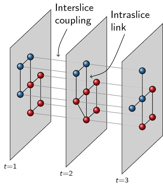
The coupling graph thus consists of three nodes and a simple line structure: 1
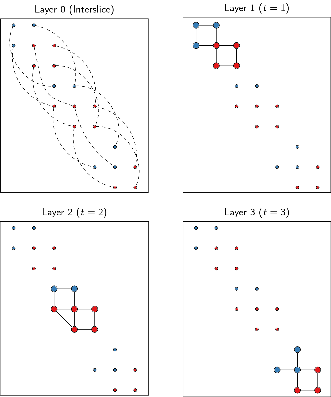
-- 2 -- 3. We convert this into layers by putting all nodes of all slices in
one big network. Each node is thus represented by a tuple (node, slice) in a
certain sense. Out of this big network, we then only take those edges that are
defined between nodes of the same slice, which then constitutes a single layer.
Finally, we need one more layer for the couplings. In addition, for methods such
as CPMVertexPartition, so-called node_sizes are required, and for
them to properly function, they should be set to 0 (which is handled
appropriately by the package). We thus obtain equally many layers as we have
slices, and we need one more layer for representing the interslice couplings.
For the example provided above, we thus obtain the following:
To transform slices into layers using a coupling graph, this package provides
layers_to_slices(). For the example above, this would function
as follows. First create the coupling graph assuming we have three slices
G_1, G_2 and G_3:
>>> G_coupling = ig.Graph.Formula('1 -- 2 -- 3');
>>> G_coupling.es['weight'] = 0.1; # Interslice coupling strength
>>> G_coupling.vs['slice'] = [G_1, G_2, G_3]
Then we convert them to layers
>>> layers, interslice_layer, G_full = la.slices_to_layers(G_coupling);
Now we still have to create partitions for all the layers. We can freely choose here to use the same partition types for all partitions, or to use different types for different layers.
Warning
The interslice layer should usually be of type
CPMVertexPartition with a resolution_parameter=0 and
node_sizes set to 0. The G.vs[node_size] is automatically set to 0
for all nodes in the interslice layer in slices_to_layers(),
so you can simply pass in the attribute node_size. Unless you know what
you are doing, simply use these settings.
Warning
When using methods that accept a node_size argument, this should
always be used. This is the case for CPMVertexPartition,
RBERVertexPartition, SurpriseVertexPartition and
SignificanceVertexPartition.
>>> partitions = [la.CPMVertexPartition(H, node_sizes='node_size',
...                                          weights='weight', resolution_parameter=gamma)
...               for H in layers];
>>> interslice_partition = la.CPMVertexPartition(interslice_layer, resolution_parameter=0,
...                                                   node_sizes='node_size', weights='weight');
You can then simply optimise these partitions as before using
optimise_partition_multiplex():
>>> diff = optimiser.optimise_partition_multiplex(partitions + [interslice_partition]);
Temporal community detection
One of the most common tasks for converting slices to layers is that we have
slices at different points in time. We call this temporal community detection.
Because it is such a common task, we provide several helper functions to
simplify the above process. Let us assume again that we have three slices
G_1, G_2 and G_3 as in the example above. The most straightforward
function is find_partition_temporal():
>>> membership, improvement = la.find_partition_temporal(
...                             [G_1, G_2, G_3],
...                             la.CPMVertexPartition,
...                             interslice_weight=0.1,
...                             resolution_parameter=gamma)
This function only returns the membership vectors for the different time slices, rather than actual partitions.
Rather than directly detecting communities, you can also obtain the actual
partitions in a slightly more convenient way using
time_slices_to_layers():
>>> layers, interslice_layer, G_full = \
...               la.time_slices_to_layers([G_1, G_2, G_3],
...                                             interslice_weight=0.1);
>>> partitions = [la.CPMVertexPartition(H, node_sizes='node_size',
...                                          weights='weight',
...                                          resolution_parameter=gamma)
...               for H in layers];
>>> interslice_partition = \
...               la.CPMVertexPartition(interslice_layer, resolution_parameter=0,
...                                          node_sizes='node_size', weights='weight');
>>> diff = optimiser.optimise_partition_multiplex(partitions + [interslice_partition]);
Both these functions assume that the interslice coupling is always identical for all slices. If you want more finegrained control, you will have to use the earlier explained functions.